Focusing on Ultrasonic

With the start of 2014 PCTE is looking forward to introducing the next generation of Proceq equipment. We have received and trained on the new Pundit PL 200PE ultrasonic system with both ultrasonic pulse velocity [UPV] and pulse echo testing. We will soon be launching the next generation of the ProfoMeter cover meter also.

As we have been working hard improving our knowledge this issue of Construction NDT delves into more advanced applications of both ultrasonic tests with a case study for UPV tomography. For pulse echo we will be reviewing different scan formats that can be collected, and when and how different processing methods can be applied to refine data for the easiest and most clear interpretation.

Sonic Pulse Velocity Case Study

Ultrasonic pulse velocity(UPV) be used to create tomograph slices through structures such as walls and columns. In this case study a variant of UPV called Sonic Pulse Velocity (SPV) was used to create a tomogram of a dam wall to find defects within it. 

SPV is very similar to UPV in that it is a time of flight method however instead of using a transducer as the source of the ultrasonic wave a strike from an impacter is used. This strike generally has lower frequency components which make it ideal for thicker elements. It also alleviates the need to couple the source to the element.

A tomogram is constructed using many SPV ray paths. During the calculation of the Pulse Velocity over one ray path the velocity represents the average speed of the wave over its path. However the wave itself may speed up or slow down dependent on the changeable material properties. For example the wave may be slowed by low quality or damaged material.

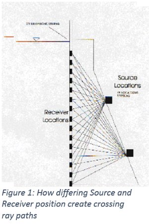
Where we only have one ray path the position of the defect is unknown. However by crossing ray paths a picture can be drawn of where the wave is slow. For example say a Pulse Velocity is taken and it is slightly slower than average. By testing a cross ray paths perpendicular to the first over the beginning, middle and end of the original ray path, it could be determined where the wave has been slowed (ie at the beginning, middle or end of the original ray path). The picture created is known as a tomogram.

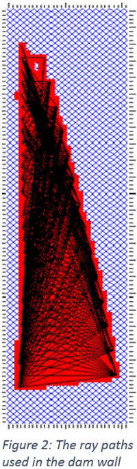
In the dam example characteristics of the dam were used to expedite the process. Firstly an impacter was built using a solenoid which could be rolled down the wall using a rope and pulley. Secondly as the other dam wall was submerged the receiver used was actually a hydrophone. The water in the dam acts as the couplant and therefore again this was just lowered using a rope and pulley.

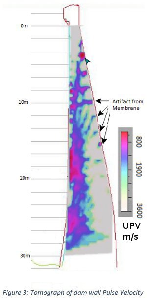
A test program was designed whereby the impacter and hydrophone were lowered to a number of different positions, creating a large number of crossed ray paths. In this way a comprehensive tomogram could be created.Once all of the data was collected a software suite programmed to create the tomogram was used to calculate the localised SPV of the dam wall and convert this to a colour coding overlayed on the schematic of the dam wall.

Using this image the area of damage were easily visible. The red/pink areas on the image to the right represent the damaged areas. On the outer side of the wall (i.e. left side) large areas of damage can be noted. On the inner side localised damage is noted at the top. The 4 artefacts noted are lower velocity points cause by air pockets in the membrane and not from damage to the wall. 

Ultrasonic Pulse Echo Testing Terminology 

Ultrasonic pulse echo testing and tomography offer many new possibilities for defect location and imaging of the internal structure of a concrete structure. In selecting a suitable system for testing and the subsequent interpretation of collected data it is important to understand some of the terminology used during scan collection, and also the exact effects and limitation of processing that can be applied to raw data.

A-Scan

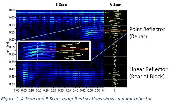
A-Scan data is the signal strength vs time of reflections at a single location on the structure after an ultrasonic pulse is applied, which is best thought of as indicating when materials change and at what depth. A-scans are typically used to measure the distance of the first reflector in the structure. This may be the rear side of the element, or a void or delamination earlier than that

At the right of the image below is the A-Scan taken at 0.5m along the length of the structure, the dotted line indicates the exact location of this single scan. Note the strong reflection at 0.15 m depth which is caused by a point reflector, and the second strong reflection around the 0.42 m mark from a linear reflector, in the A-scan it is impossible to distinguish between the two.

B-Scan

Raw B-Scan data acts as a map of the amplitude of multiple A-Scans, typically along a line on the structure. An A-Scan should be recorded every 10mm if SAFT processing is applied, or at a spacing suitable to locate the minimum defect of concern.

The image above shows how the B-Scans will show evidence of point reflectors in scans before and after a transducer passes them. This shows as a hyperbolic trace in the B-Scan and there is also a line pattern caused by compression and tension changes that carry the wave.

Raw B-Scans are good for locating linear reflectors such as the back of the slab or a clean delamination, but if point reflectors are visible processing can increase the clarity providing scans are close enough together to apply SAFT processing. Envelope processing can be used with any scans to remove the line pattern.

Synthetic Aperture Focussing Technique

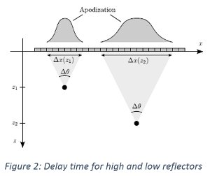
The synthetic aperture focusing technique (SAFT) is a method of processing B-scan images, which as discussed previously are an intensity map formed of A-Scan data. The process acts analogously to the way a lens will focus light from many direction to a single focal point. To perform this calculation for a single point in the B-Scan all the A-Scans of the whole B-Scan length have a delay applied according to their distance from the point being processed, then the strength of these reflection are summed at to determine the total reflection energy at that point. 

Where there is a real reflector at this point the reflection is visible in all scans at the same time after delay, and it will reflect strongly in the SAFT processed B-Scan. The image shows how the delay applied will differ for shallow and deep points.

To apply SAFT to a scan every point has the same process applied, and now point reflectors will be properly resolved into a single location, the slope visible to the side of the point reflector removed as they do not appear in the majority of the summed delay scans for that point and linear reflections remain visible as their reflection strength will remain constant.

Envelope Processing

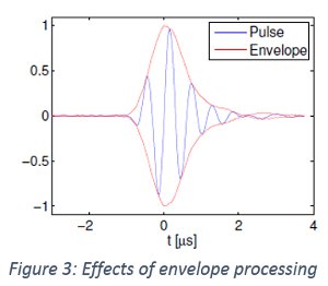
Ultrasonic data reflects the rapid change between compression and tension in the material that carries the wave. Envelop processing sums the amplitudes so that the line patterns created by this signal are removed. The image at right best reflects what this processing does and its results on a scan.

Effects of data processing

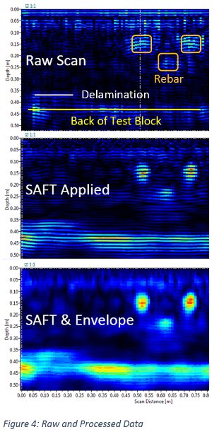
The image below shows a test block with delamination at the left close to the rear of the slab, then three reinforcing bars located close to the top surface of the slab, each processing step is included to show the different effects. You can clearly see all three bars, the delamination and the back wall in every data step, but clarity is improved when processing is applied.